|
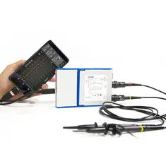
For about 100 euros you get a two channel USB oscilloscope with a bandwidth of 20 MHz and a sampling rate of 50 Msa/s, a datalogger, a function generator and a four channel logic analyzer. A set that is more than worth a comprehensive review. |
Introduction to the OSC482X from LOTO Instruments
The manufacturer and the types
This USB oscilloscope in an original design is developed by the Chinese LOTO Instruments and sold through the well known internet channels. In the series OSC482 seven types are available. All types have a bandwidth of 2 x 20 MHz, a sampling rate of up to 50 Msa/s and can work with all versions of Windows via the software OSC48XXC.exe.
A short overview of the differences between the types:
- OSC482:
Basic model without extras. - OSC482M:
Basic model + Android support. - OSC482S:
Basic model + function generator module. - OSC482L:
Basic model + logic analyzer module. - OSC482X:
Basic model + function generator module + logic analyzer module. - OSC482F:
Basic model + Android support + function generator module + logic analyzer module. - OSC482H:
Basic model + Android support + function generator module + logic analyzer module + differential input module.
The delivery of the product
Compared to the low Chinese packaging standards, the OSC482X is delivered in a very neat way. All components are in a sturdy cardboard box. The USB oscilloscope is placed in the upper compartment, well protected against possible damage of the package. The lower compartment contains all cables and the function generator module. Manual and software are not included, you need to download them from the internet.
 |
| The way the oscilloscope is delivered. (© 2020 Jos Verstraten) |
In the figure below, all components of the OSC482X are presented:
- 1
The USB oscilloscope OSC482X. - 2
Two 1/1 and 1/10 BNC test leads of 110 cm length with 60 MHz bandwidth in the 1/10 position. - 3
A 90 cm long BNC test lead with crocodile clips. - 4
A USB-A to USB-B cable of 120 cm. - 5
A 30 cm long six core cable for the logic analyser with a DE-15 connector on one side and six miniature clips on the other side. - 6
The digital function generator module with sine output up to 13 MHz, triangle output up to 8 MHz and square output up to 1 MHz.
 |
| The components present in the OSC482X package. (© 2020 Jos Verstraten) |
The USB oscilloscope is housed in a remarkable housing that consists of two parts that click into each other via a connector. In the left part is the USB control and the memory containing the firmware, in the right part the analog input circuits and the ADC. The housing consists of aluminum and a protection made of plastic.
The complete device measures 14.0 cm by 9.5 cm by 2.3 cm and weighs 210 g.
On the front panel are the two BNC connectors for the two input channels and a DE-15 connector for connecting the function generator, the logic analyzer cable or the differential input module.
The left BNC connector is connected to channel A. This is important to remember because the oscilloscope only triggers on the signal connected to this channel.
On the back panel is a USB-B connector to connect the oscilloscope to your PC or laptop. A red and green LED shows the status of the device.
 |
| The housing of the OSC482X. (© 2020 Jos Verstraten) |
According to the manufacturer, the OSC482X has the following specifications:
- Vertical resolution: 8 bit hardware, 13 bit oversampling via software
- Sampling rate: 50 MSa/s
- Interpolation between samples: linear or sin(x)/x
- Acquisition modes: normal, high resolution, top detection
- Screen layout: 10 div horizontally and vertically
- Analogue bandwidth: 2 x 20 MHz
- Input coupling: AC/DC
- Input impedance: 1 MΩ // 25 pF
- Input sensitivity: 20 mV/div ~ 2 V/div in 7 steps
- Maximum input voltage: ± 60.0 V
- Time base: 25 s/div ~ 50 ns/div in 24 steps
- Trigger source: Channel A rising or falling edge
- Trigger modes: normal or single
- Voltage measurements: peak-to-peak, maximum, minimum, average, RMS
- Time measurements: period, positive pulse width, negative pulse width
- Other measurements: frequency, rise time, duty-cycle
- Fast Fourier Transform: 1,024 ~ 16,000 points
- FFT algorithms: Rectangle, Hanning, Hamming, Blackman
- Mathematical functions: A+B, A-B, A●B, X/Y
- Screenshots: JPG/GIF/BMP format
- Recorder: 20 GB max. file size
- Datalogger sampling interval: 1 s ~ 1 h
- Datalogger logging duration: 1 m ~ 73 h
- Protocol decoding: UART/RS-232/485/422, I²C,CAN
- Operating system: Windows XP, Win7, Win8.1, Win10 (32 bit and 64 bit)
- Power supply: 5 Vdc, 250 mA via USB cable
The photo below shows the two sides of the two PCBs in the case. The left PCB is a USB interface used by various manufacturers of USB oscilloscopes. This left PCB can for example also be found in the SainSmart DS802 USB oscilloscope. This PCB is based on the Cypress CY7C68013A microprocessor with integrated USB 2.0 protocol. The board also contains a Microchip EEPROM 24lC64, which probably stores the firmware of the oscilloscope.
The right PCB is specific for the OSC482X. There is surprisingly little electronics on this board. The heart of the electronics is a MXT2088 from MXTronics Corporation. This is a two channel 8 bit ADC with a maximum sampling rate of 100 MSa/s and integrated sample&hold. Furthermore we find two CD4052 analog multiplexers and two relays on the PCB.
 |
| The two PCBs in the OSC482X. (© LOTO Instruments) |
The software and the manual
Download two programs and a USB driver
To use all the possibilities of the OSC482X you need two programs, one for working as an oscilloscope and one for working as a data logger. Of course you need to load a driver that provides the communication via USB to your PC.
For your convenience, we have copied these files to three folders on our Google Drive account. You can download them there:
How that is done depends a bit on the version of Windows you are working with. The method we describe works, as far as we know, for all versions. Connect the OSC482X to a USB connector of your PC or laptop. Some versions of Windows will install the driver automatically, some will require you to do that manually.
Go via the 'Control Panel' to 'Device Manager'. In the list of connected devices, under 'Other devices', you will see the oscilloscope as 'OSC802'. Click on this device. In the popup window, select 'Update Driver Software'. In the next window, select the folder on your hard disk where you extracted OSC_Driver. Windows will find the necessary drivers and install them in the system folder of your PC.
Starting the programs
The two programs for the oscilloscope and datalogger functions are called respectively:
- OSC48XX.exe
- OSC48XX recorder.exe
Both programs do not need to be installed in Windows, they work completely independently. Double clicking on the file name is enough to start the programs.
Oscilloscope for Windows: OSC48XX.exe
Preliminary remarks
This review is based on version 5.80.0 of OSC48XX.exe. The software has a lot of features, some are useful, some are quite far-fetched. It would be going too far to describe all those options in detail in this review/test. We assume that you don't have to examine data buses very often. That is why we limit ourselves to describing how this oscilloscope performs in daily work, making two signals visible.
The additional hardware that comes with it, the function generator and the logic analyzer, is reviewed in a separate article on this blog.
The screen of the oscilloscope
After starting the program, the screen of your PC changes into an oscilloscope, see the figure below. To show the quality of the OSC482X, we have connected a 1 kHz sine wave and a square wave on both channels. These signals look great!
The designers assumed that you only want to see the most frequently used buttons on your screen. That's why a lot of settings are hidden behind tabs. Because familiar buttons that you see on a 'real' oscilloscope are now missing, the user interface of this oscilloscope is not very user friendly. It really takes a while to get used to it!
To the left of and below the oscillogram window are two scales, calibrated in voltage and in time. Even lower below this window, the most important parameters of the two signals, such as voltages and times, are numerically displayed.
 |
| The user interface of the OSC482X oscilloscope. (© 2020 Jos Verstraten) |
In the figure below we have enlarged the control panel of the two input channels. The first thing that stands out is that both channels have only seven sensitivity positions: 20 mV/div ~ 50 mV/div ~ 100 mV/div ~ 0.2 V/div ~ 0.5/div ~ 1 V/div ~ 2 V/div.
This is very little, a normal oscilloscope has at least 12 positions and goes beyond the OSC482X on both the most sensitive and least sensitive side. Fortunately, this is somewhat compensated by the presence of two slider potentiometers, with which you can set the sensitivity between the values of the rotary switch. In this way you can increase the sensitivity to 10 mV/div. The exact value of the sensitivity appears in a box. In the example below, the sensitivity of channel B is set to 1.332 V/div. Use the knob with the counterclockwise arrow on it to restore the calibrated sensitivity of the rotary switch.
With the buttons marked 'chA' and 'chB' you switch both channels on or off. The buttons 'AC/DC' are of course known from every oscilloscope. With the button 'baseline' the software puts two horizontal lines on the screen at the 0 V references of both channels.
With the button next to the notation '1X' you can add the attenuation of a probe in the signal calculations. This button has four positions: 1X ~ 10X ~ 100X ~ 20X.
At channel B you will see another button with a digital signal drawn next to it. With this button channel B becomes the logic analyzer, read the separate article.
 |
| The control panel of the vertical channels. (© 2020 Jos Verstraten) |
Finally, at channel A, you will see a button 'Persistence' (next to the 'baseline'). This option displays the data of channel A superimposed on the screen. The old trace will not be replaced by a new trace, but the traces will be written on top of each other. This way, the maximum value of possible noise on the signal is made more visible, see figure below, where the same signal above with and below without this option is shown. For some reason, this option only works on channel A.
 |
| The effect of the 'Persistence' on channel A. (© 2020 Jos Verstraten) |
As shown in the figure below, the time base rotary switch has only eight positions: 0.5 ms/div ~ 0.2 ms/div ~ 20 μs/div ~ 4 μs/div ~ 1 μs/div ~ 0.5 μs/div ~ 0.2 μs/div ~ 0.1 μs/div. However, with two additional positions, you can click on a frame which allows you to select from 16 speeds on the low side and from only one speed on the high side: 50 ns/div.
What the use is of time base speeds of more than 1 s/div is a mystery to us. To view such slow varying signals you better turn on the 'Paperless Recorder'.
The high side is of course much more interesting. A fastest setting of 50 ns/div is still quite slow, but fortunately there is also a slide potentiometer available with which you can increase the speed to 10 ns/div. With the knob with the counterclockwise arrow on it, you can go back to the calibrated value of the rotary switch.
With the button 'auto' the OSC482X searches for the most suitable time base speed itself. Approximately five periods of the signal will then appear on the screen.
 |
| The time base control panel. (© 2020 Jos Verstraten) |
The trigger function is a very important function in any oscilloscope. Thanks to the triggering, you get a completely still image on the screen. Most oscilloscopes pay a lot of attention to this function, so you can set exactly what you want to see on the screen and how you want to see it. It is quite strange that the designers of the OSC482X pay hardly any attention to this function. The trigger window is hidden under the tab 'Tri' of channel A. When you open this box, you will notice that you can only trigger on channel A and that there are only two options:
- Trigger on front or rear edge.
- Normal or Single.
With this last setting, the oscilloscope waits for a signal level that matches the trigger level and then writes one trace on the screen. You can set the trigger level by moving a blue triangle, to the right of the oscillogram window, up and down with the mouse.
 |
| The trigger offers very few settings. (© 2020 Jos Verstraten) |
In the picture below, we showed this image jitter by using the 'Persistence'-option of channel A. You see a signal of 100 kHz, the various traces that are written on the screen give an impression of the size of the image-jitter.
 |
| The size of the image jitter at 100 kHz. (© 2020 Jos Verstraten) |
With this setting you can determine how the digital samples are put on the screen:
- Normal:
This is the default setting where all samples are translated to analog values that are drawn as dots on the screen. These dots are connected to each other by lines (read more). - Peak-Detect:
This involves sampling at the maximum speed and searching for the maximum value in each sample interval. This is put on the screen. However, for most signals you will not see any difference between 'Normal' and 'Peak-Detect'. This mode is recommended if you need to look for narrow glitches in a signal. - High-Res:
This mode uses oversampling techniques. Between two real samples a number of extra samples are calculated that appear on the screen. This way the resolution can be mathematically increased from 8 to 13 bit. - Sine:
The successive samples on the screen are connected with sinusoidal line segments via a mathematical interpolation algorithm. - Linear:
Here the successive samples are connected with straight lines.
 |
| The acquisition window and the difference between sine and linear interpolation. (© 2020 Jos Verstraten) |
The tabs around the vertical settings
Seven tabs with various functions
On the right side of the control panels of the vertical channels you will see seven tabs. These have, from top to bottom, the following functions.
A
Put the controls of channel A in the window.
Tri
Opens the trigger window, which has already been discussed.
Pro
Stands for 'Probe'. You can adjust the scaling of the oscilloscope to a special current probe that you connect to channel A. If this probe delivers 100 mV/A you can set that in this window. The numerical scale to the left of the oscillogram window will then be displayed in A instead of V.
B
Put the controls of channel B in the window.
Lgc
Stands for 'Logic', has something to do with the logic analyser, read separate article.
Dif
Has a function when you connect a differential probe to the B input, read separate article.
Pro
Scaling for a special probe connected to channel B.
The tabs around the time base setting
Eight different functions
The time base control panel has no less than eight tabs on the top and right side that all enable a certain function.
Sett
Put the time base controls in the window.
Exte
Important when setting the function generator, read separate article.
Deco
Abbreviation of 'Decoder'. Decodes serial data streams of different protocols, so that the oscilloscope triggers them.
Adva
Stands for 'Advanced'. With this option you can put up to 2 x 12 parameters of the two input channels enlarged on the screen, the so-called 'Measurement Magnifier'. Some of these parameters: RMS value, top value, peak-to-peak value, frequency, period, duty-cycle, rise time. With this tab you also make the 'Deep Measurement' active. The software then calculates the time between the zero crossings of the signal and puts these times in a table.
 |
| The window in which you switch on the 'Advance' measurement values. (© 2020 Jos Verstraten) |
Stands for 'Reference comparison'. This option allows you to insert an oscillogram previously saved as a JPG file into the current oscillogram, so you can compare both properly. With a number of slider potentiometers you can adjust the position and size of the second oscillogram, so you can move it exactly over the first one if you want.
 |
| The window in which you enable the 'Reference comparison'. (© 2020 Jos Verstraten) |
Put the time base controls in the window.
Car
You can define the sampling rate and memory size of the buffer.
Rec
Obviously stands for 'Recording'. With this option you can record the events on the screen in a video. You can set the number of frames you want to record. After a click on the 'REC' button an automatically generated filename will be suggested. After a click for approval the recording will start. In the video, the full user interface of the oscilloscope is recorded, so you can see which settings the device had during recording.
Unfortunately, the recording has its own format, so you can't play the video without the program. Why not use .MP4?
 |
| Setting up a video. (© 2020 Jos Verstraten) |
The display options
A toolbar with twelve options
Between the oscillogram window and the control panels is the twelve option toolbar shown in the figure below. The names we have written next to the icons will in most cases make it clear what the option stands for.
 |
| The button bar with display options. (© 2020 Jos Verstraten) |
With this option, two horizontal and two vertical cursors appear on the screen which you can move with the mouse. This way you can measure the time or voltage between the two cursors. These relative measurements are displayed with the delta symbol ∆.
Fast Fourier Transform
This option allows you to display the frequency composition of a periodic signal in a graph. In the example below you can see for example the fourier analysis of a symmetrical square wave with a frequency of 10 kHz.
 |
| The FFT analysis of a 10 kHz square wave.. (© 2020 Jos Verstraten) |
This language error is in the software! This option is only available if both channels are active. You can perform mathematical operations on the two signals:
- A + B
- A - B
- A ● B
- X/Y Plot (Lissajous)
With this last option, the time base is switched off and the horizontal deflection is taken care of by channel B. You then get the famous lissajous figures on the screen: circles, ellipses and lemniscates. This allows you to study the phase and frequency relationship between the two signals. Noteworthy is that the X/Y plot is projected over the existing screen, see the figure below
 |
| A lissajous figure in X/Y Plot mode. (© 2020 Jos Verstraten) |
A very useful feature! If you click this icon once, twice or three times, you can quickly vary the sensitivities of the two channels and the time base with the wheel of your mouse.
Paperless Recorder for Windows: OSC48XX recorder.exe
Introduction
This program is intended for viewing very slowly changing phenomena, such as the output voltages of sensors. The user interface is adapted as much as possible to that of the oscilloscope. We will discuss version 1.0.2.
You can only configure the program when the recorder is stopped. You can set the sensitivity of both channels, the total time of the recording and the interval between samples.
 |
| The user interface of Paperless Recorder for Windows. (© 2020 Jos Verstraten) |
Four sliding potentiometers are available for this purpose at the top right of the window. You can vary the total time from one minute to 72 hours and 60 minutes, i.e. 73 hours. The interval between two samples ranges from one second to 60 minutes and 60 seconds, i.e. 61 minutes.
The sensitivities of both channels
This can be set in seven steps from 20 mV/div to 2 V/div. You can select a multiplication factor of 1X, 10X or 100X.
Acquisition mode
As with the oscilloscope, you can choose between:
- Normal.
- Peak-Detect.
- High-Res.
The toolbar
It contains some of the buttons already known from the oscilloscope, among others for saving the data as an image or text file.
The oscilloscope in practice
A very important remark
No attention is paid to it in the manual, but when measuring with the OSC482X, always remember that there is NO GALVANIC ISOLATION between the ground of the two BNC inputs and the ground of the USB output. If you apply a dangerously high voltage to one of the inputs, it can happen that this voltage is also present on the chassis of your PC. In the worst case, a very large current may flow between the ground of the BNC connectors and the ground of your PC, causing fuses to blow and thin cables to burn out. If you need to measure such voltages, always use the differential input module IDM01.

The display of 1 kHz signals
In the seventh illustration of this article we have put signals of 1 kHz on the screen and they look perfect. But how does the OSC482X behave when we push the limits of its specifications? We present a few examples to give you a good impression of the quality of this USB oscilloscope.
A sine wave of 20 MHz
The analog bandwidth is specified as 20 MHz, so we were curious how a sine wave signal would be displayed at this frequency. The horizontal dotted lines in the illustration below represent the peak-to-peak value of a 1 kHz sine with the same amplitude. You notice that the 20 MHz signal is hardly weakened, so the bandwidth is fine. What does avenge with such a signal is the limited sampling rate of only 50 Msa/s. Few samples are taken per period from a 20 MHz signal. This signal was sampled with sine interpolation and high-res acquisition. In the inset, the same signal is displayed on a oscilloscope with a sampling rate of 1 Gsa/s.
The OSC482X did not numerically display the frequency of this signal properly: 13.714 MHz instead of 20 MHz.
 |
| Display of a 20 MHz sine wave signal. (© 2020 Jos Verstraten) |
In the picture below we show the results of a sine wave and a saw tooth of 1 MHz. The ringing visible on the saw tooth is really not on the signal, but is generated by the oscilloscope itself. With these signals, the frequency is measured well.
 |
| Display of 1 MHz signals. (© 2020 Jos Verstraten) |
Then we connected a square wave of 100 kHz to the two oscilloscopes. You can see the result in the picture below. The inset shows the image on our 100 MHz oscilloscope as a reference.
 |
| Display of a 100 kHz square wave. (© 2020 Jos Verstraten) |
Digital oscilloscopes are notorious for contaminating small signals with spikes and other digital junk. We offered an absolutely pure sine wave with a frequency of 1 kHz and an RMS value of only 10 mV to both devices. You see the result on the picture below. The OSC482X performs better than our Hantek 100 MHz oscilloscope. Less contamination on the signal!
 |
| Display of a 10 mV sine signal. (© 2020 Jos Verstraten) |
Our opinion on the OSC482X from LOTO Instruments
If you take the occasional small jitter in the image at deflection speeds of more than 0.2 ms/div for granted, the OSC482X is an excellent usable USB oscilloscope for the hobby electronics enthusiast. The way the user interface is designed is a bit strange with functions hidden at rather unusual places, but that is a matter of getting used to. Of course, you cannot compare the performance with a 100 MHz oscilloscope with a sampling rate of 1 Gsa/s that is three times more expensive. Moreover, think of what you will get for your hundred euros extra: a good software datalogger, a real function generator and a four-channel logic analyzer.

OSC482X Digital Portable Oscilloscope